
Extending the Flight Search Engine: Time, Cost, and Feasibility constraints
Graph series - part 4

In the previous article, we built a structural flight search engine capable of traversing an aviation graph and enumerating valid routes between airports. The system was correct — but incomplete. Pure connectivity ignores the realities that make flight search non-trivial: time, physical distance, cost, and feasibility constraints.
In this article, we extend the engine in two fundamental ways. First, we introduce a data provider abstraction, decoupling traversal logic from the underlying data source. We begin with a local OpenFlights dataset, but the engine now depends only on a provider interface — allowing live API-backed implementations to be substituted without modifying search logic. The system becomes extensible through abstraction rather than conditionals.
Second, we enrich the domain model itself. Flights become timezone-aware events. Travel duration is derived from airport coordinates and aircraft cruise speeds. Layovers are validated against feasibility rules. Pricing becomes a structured responsibility of the provider rather than a hardcoded afterthought.
These changes transform the problem from structural traversal into constrained itinerary evaluation. The traversal strategy remains depth-aware, but the cost of evaluating each branch increases significantly. This performance regression is intentional — the natural consequence of introducing realism. In the next article, we will address how to make this richer system efficient.
Designing for Substitution - introducing data providers
In the previous iteration of the engine, traversal and data access were tightly coupled. The graph was constructed from a local dataset, and the search algorithm operated directly on that structure. While functional, this approach implicitly assumed that the data source was static and local.
Real flight search systems do not operate this way. They query distribution systems, APIs, and live availability services. If the engine is to evolve toward real-world integration, the abstraction boundary must shift.
We introduce a FlightDataProvider interface. The engine no longer knows how flights are stored or retrieved. It requests outbound flights for a given airport and departure time, and it requests a price for a completed route. That is the entirety of the contract.
Conceptually, the dependency direction changes:
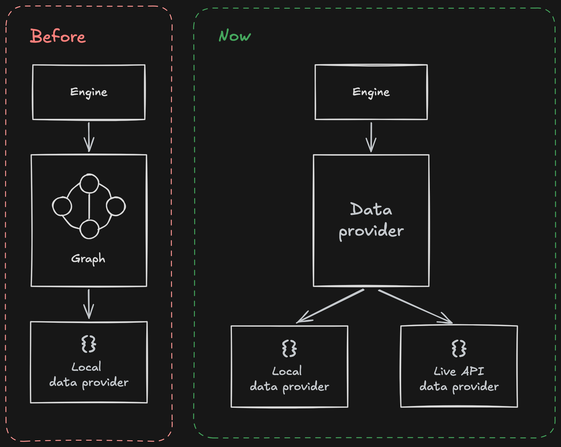
Before, the engine depended directly on the graph and its concrete dataset. Now it depends on an abstraction. The concrete provider — whether local or API-backed — is selected at composition time.
The provider interface is intentionally narrow. It does not expose storage concerns or transport mechanisms. It exposes only the capabilities required for search. This ensures that substitution happens through implementation, not conditional branching.
Instead of embedding logic such as:
if provider_type == "local":
    ...
elif provider_type == "live":
    ...
We compose the engine with a concrete implementation:
provider = OpenFlightsProvider(data_dir)

routes = find_flight_routes(
    origin="JFK",
    destination="SYD",
    provider=provider,
    departure_time=departure_time,
    max_legs=3,
    max_routes=5,
)
Replacing the data source is as simple as instantiating a different provider:
provider = RealProvider(api_key=...)The engine itself remains unchanged.
This design follows established principles:
Liskov Substitution Principle — any provider must be replaceable without affecting correctness.
Open/Closed Principle — the engine is open to extension, closed to modification.
Dependency Inversion — high-level traversal depends on abstractions, not concrete data sources.
With this boundary in place, traversal logic, time modelling, feasibility constraints, and pricing can evolve independently of how data is sourced. That separation is the structural foundation for the remainder of this article.
Modelling Real-World Constraints
With the provider abstraction in place, we can now make the engine behave more like a real flight system.
Our OpenFlightsProvider is not a live scheduling backend. It is a deliberate approximation. We simulate daily departures at fixed times. We calculate travel duration from airport coordinates and aircraft cruise speeds. We attach structured pricing to completed routes. We enforce layover feasibility rules.
The goal is not to replicate airline reservation systems. The goal is to introduce the kinds of constraints that make flight search non-trivial — while remaining deterministic enough to run locally without relying on a live API.
We want something close enough to reality to reason about scheduling, cost, and optimisation. That is the purpose of this provider.
Time as a Constraint
Once we introduce departure and arrival times, routes stop being abstract paths.
Each flight now has:
A departure datetime in the origin airport’s local timezone
An arrival datetime in the destination timezone
A calculated duration
We simulate a fixed daily departure time in the origin airport’s local timezone. Arrival time is derived from the computed travel duration. Internally, we normalise through UTC to ensure timezone transitions are handled correctly.
The important shift is this: connectivity is no longer sufficient. A connection must also be feasible in time.
Layover validation enforces this. The next flight must depart after arrival, and the layover must fall within acceptable bounds. At each recursive step, we carry forward not only the current airport, but the current arrival time.
The search state becomes richer: it is no longer just (airport), but (airport, time).
Physical Reality as a Constraint
In the structural engine, every edge was effectively weightless. Now, travel time is derived from physical distance.
We compute distance between airports using their latitude and longitude. That distance is combined with an aircraft-specific cruise speed to determine airborne time, and a small ground buffer is added to approximate taxi, climb, and descent.
Different aircraft types travel at different speeds. A long-haul wide-body does not behave like a regional turboprop. Even in a simplified model, this matters.
This introduces two important changes:
Duration is no longer constant or arbitrary.
Evaluating a route now requires real computation.
Each candidate route requires distance calculations, speed resolution, and datetime arithmetic. These operations accumulate quickly as the search deepens.
Cost as a Constraint
We also introduce pricing, and importantly, pricing belongs to the provider.
The search engine does not calculate fares itself. It requests a price for a completed FlightRoute. For the OpenFlightsProvider, we simulate pricing using a structured model:
A base fare
A distance-based component
A layover penalty
The result is a structured Price object attached to the route.
This keeps the pricing logic aligned with the provider abstraction introduced earlier. A future live provider could replace this synthetic pricing model with real API-backed offers — without changing the search engine.
Cost is now part of the evaluation of a route, not an afterthought.
Feasibility as a Constraint
Taken together, these constraints change the nature of the problem.
Previously, we asked:
Is there a path between A and B within N hops?
Now we ask:
Is there a feasible, time-valid, economically evaluated itinerary between A and B within N hops?
The traversal algorithm itself has not changed. We still perform depth-first search with hop limits. What has changed is the weight of each expansion. Every step now carries temporal state, physical computation, and potential pricing. We have moved from connectivity to constrained feasibility.
With time, physical modelling, and pricing integrated, the engine now produces itineraries that reflect scheduling constraints rather than simple connectivity. A truncated example output is shown below.
./run_local.sh
Skymesh provider loaded
Airports loaded: 6072
Origins with outbound routes: 3241

============================================================
Searching routes: SYD -> MEL

SYD -> MEL (1 legs, total 1h 7m)
    Leg 1: SYD -> MEL
    Airline: Qantas
    Dep: 9:00 AM, 01-03-2026 (UTC+10:00)
    Arr: 10:07 AM, 01-03-2026 (UTC+10:00)
    Total Price: USD 134.65 (Base: 50.00, Distance: 84.65, Layover: 0.00)

============================================================
Searching routes: JFK -> SYD

JFK -> SYD (2 legs, total 29h 30m)
    Leg 1: JFK -> DXB
    Dep: 9:00 AM, 01-03-2026 (UTC-05:00)
    Arr: 7:16 AM, 02-03-2026 (UTC+04:00)

    Layover: 1h 43m

    Leg 2: DXB -> SYD
    Dep: 9:00 AM, 02-03-2026 (UTC+04:00)
    Arr: 5:30 AM, 03-03-2026 (UTC+10:00)

    Total Price: USD 2,891.30
Depth-Aware Ranking and Search
In Implementing a Flight Search Engine, we introduced Iterative Deepening Depth-First Search (IDDFS) as the traversal backbone of the system. There, we explored its mechanics in detail and justified the choice in terms of hop optimality, bounded memory behaviour, and predictable expansion.
[Article 3 here]
Introducing time, distance, and pricing does not require us to change that traversal strategy. What changes is the cost of evaluating each branch and the way we rank completed routes.
IDDFS remains the backbone. The difference now lies in how we order and constrain results within each depth.
Hop Count Remains the Primary Ordering
In practical flight search, direct routes are generally preferred over multi-stop itineraries. A two-hour direct flight should not be outranked by a slightly faster two-stop alternative.
For that reason, hop count remains the primary ordering constraint.
We search depth by depth:
First, all 1-leg routes
Then, 2-leg routes
Then, 3-leg routes
Within each depth, we rank routes by total duration. But we never allow a deeper route to displace a shallower one purely because it is shorter.
This preserves structural preference while still allowing meaningful ranking within the same hop count.
Sorting Once Per Depth
A naive implementation might collect all routes and perform a global sort by duration or price. That approach breaks hop semantics and introduces unnecessary computational cost.
Instead, we:
Explore all routes for a given depth limit
Sort only the routes discovered at that depth
Select up to
max_routesStop deepening once sufficient routes are found
Sorting happens once per depth — not on every append, and not globally.
This approach maintains depth priority while keeping ranking behaviour predictable and controlled.
Why Not Breadth-First Search?
Breadth-First Search (BFS) naturally finds shortest paths in terms of hop count. For purely structural traversal, BFS would be a reasonable alternative.
However, BFS maintains the entire frontier in memory. Once we introduce time-aware state — effectively (airport, time) pairs — the breadth of that frontier expands quickly.
IDDFS gives us the same hop-optimal guarantees as BFS, but with significantly lower memory overhead. We trade some re-computation for bounded memory growth. Given that each node evaluation now performs non-trivial computation, controlling memory pressure is important.
Why Not Dijkstra’s Shortest Path?
Dijkstra’s algorithm optimises for a weighted shortest path. If our objective were strictly “minimise total duration” or “minimise price,” Dijkstra would be a natural candidate.
But our problem is not purely weight-based.
We enforce layered constraints:
Maximum hop count
Layover feasibility
Provider-defined pricing
Depth-based preference (direct routes outrank multi-stop routes)
Dijkstra assumes a single monotonic weight function. Our engine applies structural limits first, then ranks within those limits.
Hop count is not just a weight — it is a boundary.
IDDFS allows us to enforce hop limits explicitly while layering duration-based ranking inside each depth. That alignment between algorithm and domain constraints is intentional.
The Backbone Remains the Same
The traversal strategy itself did not change when we introduced time, cost, and feasibility. What changed was the richness of the state propagated through recursion and the computational cost of evaluating each branch.
We did not replace the algorithm, we increased the weight of each node. That distinction becomes visible when we measure runtime.
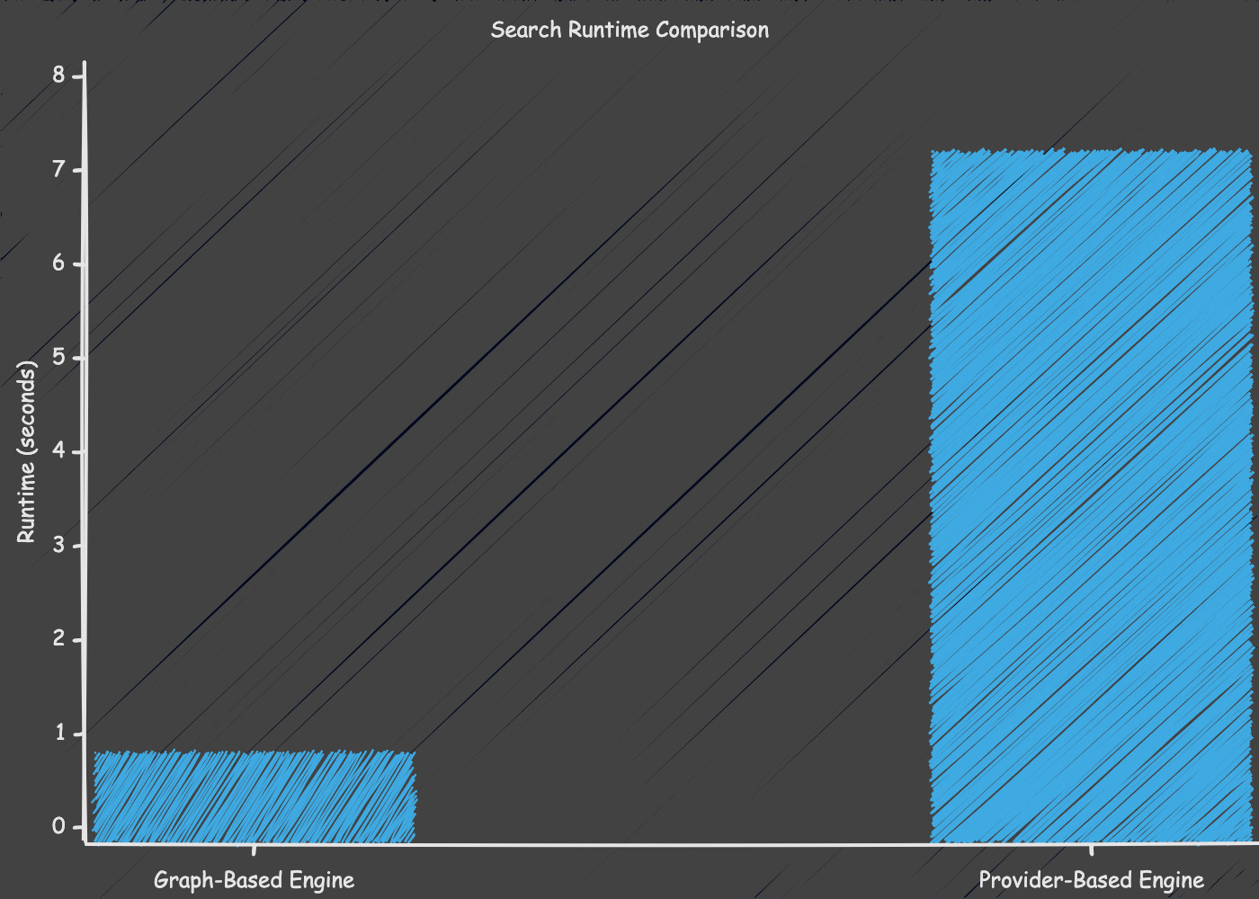
Performance Regression: Measuring the Impact of Added Constraints
Up to this point, every change we introduced was about realism — not speed. We did not alter the traversal algorithm, increase max_legs, or expand the graph. Yet runtime increased significantly.
In the structural engine, a typical search completed in under one second. After introducing time modelling, aircraft-based duration calculations, layover validation, and provider-driven pricing, the same search now takes approximately seven to nine seconds.
Nothing about the traversal strategy changed. What changed was the cost of evaluating each node.
Search Runtime Comparison
What Became More Expensive?
Each completed route now requires:
Distance calculation between airports
Cruise speed resolution based on aircraft type
Duration computation and timezone-aware datetime arithmetic
Layover validation
Provider-based pricing evaluation
These are not simple adjacency checks. They involve trigonometric functions, datetime conversions, and structured object construction. Individually small, collectively significant.
In the structural engine, evaluating a branch meant checking connectivity. In the constrained engine, evaluating a branch means simulating a flight.
Time also expands the search state. Previously, a node represented an airport identifier. Now it effectively represents (airport, arrival_time).
The same airport may appear multiple times in the search tree at different times of day, each carrying distinct feasibility implications. The graph has not grown, but the dimensionality of state has.
The regression does not stem from a more complex traversal algorithm. It stems from increased per-node computation and richer state propagation.
Having made the system more expressive and realistic, we now face the natural next question: how do we reduce this computational cost without compromising correctness? That will be the focus of the next article in this series, where we optimise this slower—but more accurate—engine.